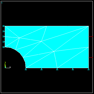
p-Method Example - When the element polynomial order is varied while solving the FEM model in order to seek suitable accuracy of the computed FEM results it is termed the p-Method. In the example below the p-method is used to determine accurate stresses in a plate with a hole.
1. Start ANSYS and select Preferences -> p-Method
2. Preprocessor -> Element Type -> Add -> Add -> select 2D triangle 146 -> OK -> Options -> Plane Stress + Thickness -> Close
This selects a p-method, plane-stress element with a given thickness which you provide as indicated below.
3. Preprocessor -> Real Constants -> Add -> Type 1 Plane 146 -> OK -> enter thickness.
Create geometry and mesh as discussed in the scf example. Add loads and bc to give the following model.

With p-method selected under preferences, the program will solve the FEM problem repeatedly, automatically adjusting the polynomial level in the elements until a user-specified solution quantity ceases to change to within some specified tolerance.
The default convergence criteria is that the total strain energy in the model stabilize to the point that its value for a new polynomial level is within 5% of the value as found using the previous polynomial level. To solve the problem using the default convergence criteria, select as before,
4. Solution -> Current LS
5. General Post Processor -> Read results, Last Set -> Plot Results
6. Contour Plot -> Element Solution ->Stress Sx
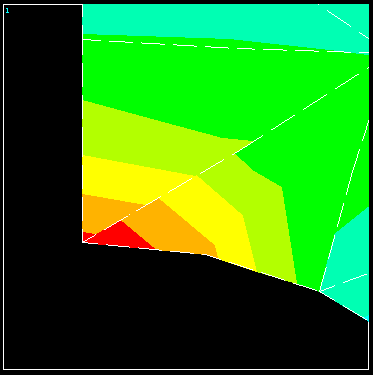
The initial p-level is set to 2 for each element. To see what the final p-levels are, select p-levels under plot results
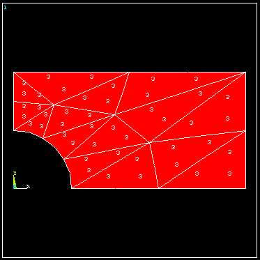
The p-level was advanced uniformly from 2 to 3 throughout the mesh. To evaluate the convergence, select p-Convergence.
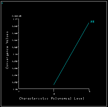
Using the default convergence criteria gives a noticeable discontinuity in stress contours across element boundaries indicating poor accuracy in the computed stresses, and the total strain energy looks as though it would continue change if the p-levels were incremented. To increase the accuracy, we will employ a different convergence criteria and solve the problem again.
The quantity of interest here is the maximum stress in the vicinity of the hole, therefore we require that the solution be repeated with increasing p-levels used for the elements until the calculated maximum stress stops changing to within some required tolerance, say 1%.
7. Preprocessor -> Loads -> Load Step Opts -> p-Method -> Convergence Criteria -> Replace -> Local for solids
Pick the node where the maximum stress will occur.
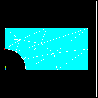
8. Select Stress Sx and change the convergence tolerance from 5% to 1% -> OK
Solve the problem again to obtain the stress contour plot shown next.
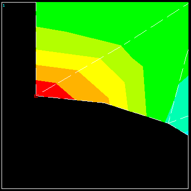
The smoothness of these stress contours gives us confidence in the solution. The p-level distribution in the mesh is shown next.
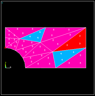
To obtain the requested accuracy, it was necessary to use p-levels of 5 in most of the elements. The convergence history of Sx at the specified node is shown next.
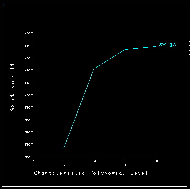
The Sx stress component at the hole is seen to converge nicely to a value in which we can have confidence. Notice that the maximum p-level available for these elements in ANSYS is 8. If using p-levels of 8 does not provide the requested accuracy, a more refined mesh must first be created and the problem solved again.