Assignments
Note that Problems are not assigned until the indicated date is for the current semester.
See Syllabus for format instuctions
HW #1 Assigned 8-27-18 Due 8-30-18
Problem 1 - A person is gripping a tube with a pair of pliers. Assume (or measure) the tube size and the plier dimensions. Make a good sketch and assign symbols to the quantities of interest. Draw a free body diagram of the pliers and draw a free body diagram of each component of the pliers.
Text Problems 2.6, 3.2
Be sure to provide a statement of the problem to be solved (the 'given'), a good sketch showing the problem, free bodies, axis systems used, etc. State what is to be found. The solution should follow with major results highlighted for easy reference by the reader.
HW #2 Assigned 8-31-18 Due 9-6-18
Text problems 3.4, 3.9, 3.15
Note: In 3.4 assume that both masses have an initial velocity of (m2)*sqrt(2*g*h)/(m1+m2).
Find the amplitude of steady state response for the system described in text problem 4.2. Repeat for the case in which the system has damping equal to 10% of critical. (See Eqns 4.9 and 4.21a)
HW #3 Assigned 9-7-18 Due 9-13-18
Text Problems 4.5 and 4.10 Note that z(t) is a displacement input and the tensile force on the right of the mass is k(z - u).
HW #4 Assigned 9-20-18 Due 9-27-18
a. Text problems 5.4.
b. Solve the problem discussed in Text example 6.3 using the MATLAB ode45 routine. Compare your solution at t = 0.2 sec to the exact solution by finding the per cent error. Also find the per cent error of the two numerical solutions given in the text.
See Our website > MATLAB for a sample program. You can cut and paste these codes from the web pages to m-files.
HW #5 Assigned 10-10-18 Due 10-23-18
a. Use Newton's second law to derive the equations of motion for the text Problem 8.3. As variables use the upward motion of G (instead of down at C) and let Theta be measured positive in a counter clockwise sense.
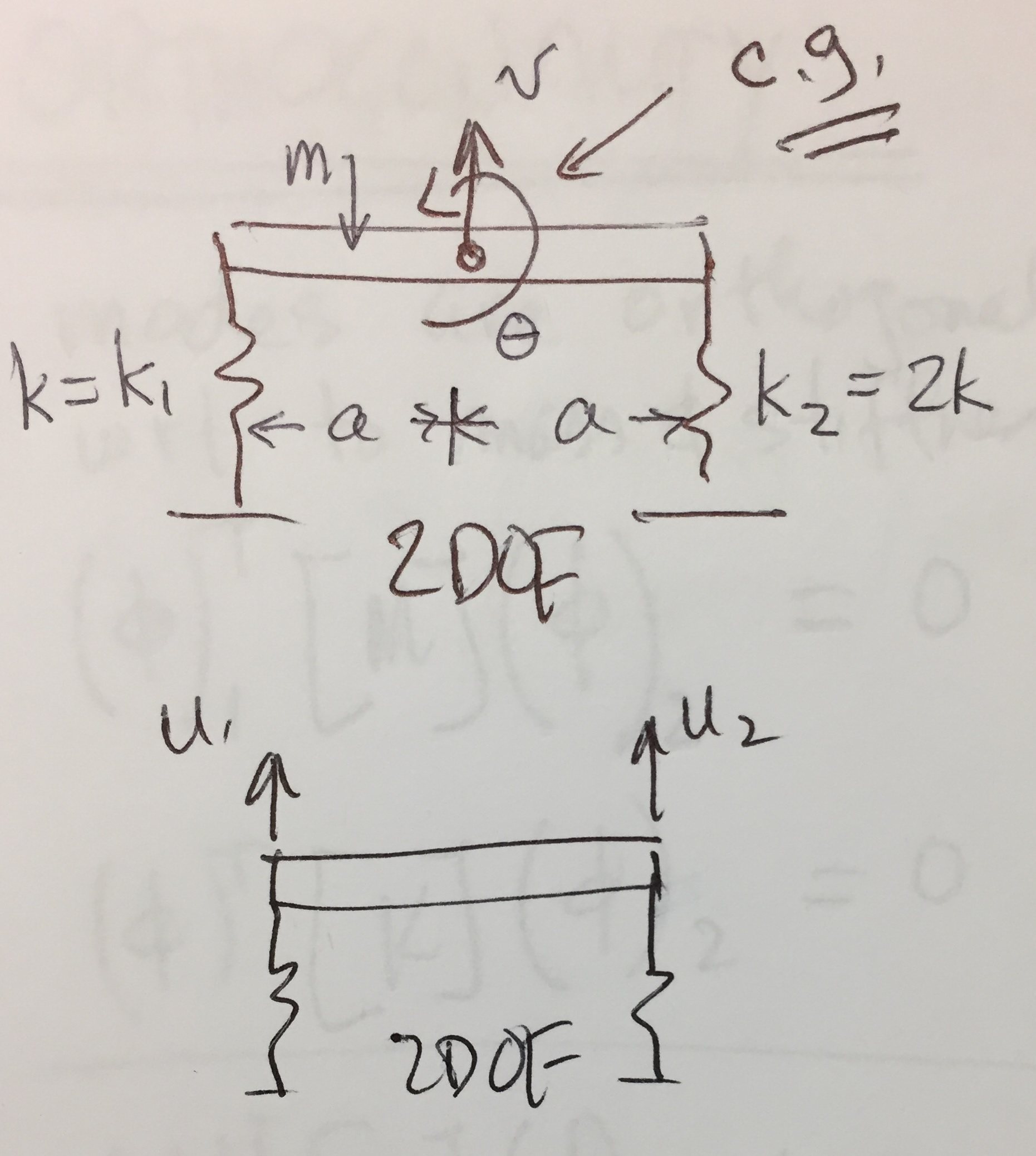
b. Derive the equations of motion for the rigid bar shown. Fig HW7 b. below.
(1) Use Newton's second law and coordinates v and theta.
(2) Use the Lagrange method and coordinates u1 and u2. (You can write expressions for ucg and theta in terms of u1, u2 and 'a'.)
HW #6 Assigned 10-11-18 Due 10-23-18
Solve Mavspace > Old Exams > Fall 2015 > Exam2 > Problems 1, 2, & 3
For Problem 3 c., use MATLAB to solve for the frequencies and mode shapes.
Normalize the modes so that the largest value is 1.0
HW #7 Assigned 10-30-18 Due 11-6-18
a. Text problem 8.12. Use the Lagrange method.
b. If mg = 200 lbf and k = 80 lbf/in , solve Example 9.1 by hand AND by using MATLAB's 'eig' function. (1) Use A = inv(M)*K, where M and K are the mass and stiffness matrices. V = mode shapes, D = (frequencies)^2
(2) Use [V,D] = eig(A) where now A = inv(K)*(M). V = mode shapes, D = 1/[(frequencies)^2]
HW #8 Assigned 10-30-18 Due 11-8-18
a. Use the equations derived in Text problem 8.9. to prepare an ODE45 simulation model for the nonlinear problem. Compute and plot the time response for initial conditions theta1 = 0 and then for initial conditionc theta2 = 30 deg. Initial velocities are zero. Run time should be long enough to observe both response frequencies.
Data: L = 12 inches, a = 7 inches, g = 386 in/s^2, m = 25 lbf/g, k = 60 lbf/in.
b. Use MATLAB to verify the frequencies and mode shapes of text Example 11.4 (Note that 'kip' means 1000 lbf.)
HW #9 Assigned 11-6-18 Due 11-13-18
a. The term project consists of your analysis and test of an object small enough to be tested (free-free boundary conditions) using a microphone and digital signal analyzer. Use the presentations from a previous semester as guidance (see Mavspace). Undergraduates work in teams of two; graduate students this is an individual project. Make sure you can use a solid modeler such as Creo, CATIA, SolidWorks. Submit your porposal consisting of a statement of what you will analyze, a hand-drawn sketch of it and who is on the team.
Send your ppt slides to lawrence@uta.edu by 5pm Monday Dec 3, 2018. We will review your work in the last class on Dec 4.
HW #10 Assigned 11-28-18 Due 12-11-18
a. Text problem 9.3. Use Newton's second law to derive the equations of motion. Use the vertical motion of the center of mass, v, and the rotation of the bar, theta, as variables instead of u1 and u2.
b. Derive the equations of motion for text problem 9.3 using the Lagrange method. Use variables v and theta as in part a.
c. Let k = m = 1 and work text problem 9.15 by hand and also using matlab.
HW #11 Assigned Due
a. Use MATLAB to find the amplitude of the response u1 in text Example 11.4 if P1 = 1000 kips. Consider the case Omega = 1.3 * Third nat freq.
Use the method discussed in class, not the mode superposition method discussed in the example. That is, given Omega, [M], [K], and {P} use MATLAB and the value given for Omega to solve for {U} and thus u1 in the matrix equation
< -Omega^2[M] + [K]>{U} = {P}
{U} = inv< >*{P}
Compare your results to those given in the last column of the table on page 347. You should get something like u1 = -0.4987 inches. Note the misprint in the book. In the problem statement Omega = 1.3* Third nat freq, but later it is printed as first nat freq. The third nat freq is the one to use.
b. The beam of Text problem 13.8 is a 10 ft long W 10 x 30 standard wide flange beam. The beam xsectn height is 10 inches, its area is 8.84 sq in. its flexural inertia 170 in^4, and its weight density is 0.284 lbf/in^3. Make a sketch to scale of the 10ft long cantilever beam.
Use the results in Text Example 13.1 to find the first three axial motion natural frequencies in R/s and in Hz.
Use the results in Text Example 13.3 to find the first three bending motion natural frequencies in R/s and in Hz.
Look up W 10 x 30 if need be and remember in the freq equations of Ex 13.1 & 13.3 that rho mass density.
HW #11 Assigned Due
a. Text problem 13.8; Use the results in Text Examples 13.1 and 13.3, not 10.1 and 10.3
b. Work through http://mae.uta.edu/~lawrence/ansys/ansys_examples.htm > Example 9.A - Truss Frequencies. Submit a copy of your input text file, documentation of the two frequencies calculated (Hz), and images of the two modes of vibration; one mode is shown in the example. Work through Example 2.A Truss1 as necessary. Access ANSYS APDL in the CAD Lab.
HW #12 Assigned Due
a. Use ANSYS APDL to compute the first three bending natural frequencies of a 10 inch long steel cantilever beam with a 2 inch wide x 0.25 inch high cross section. Use models which have 5 nodes along the length, then 10 nodes, and then 20 nodes and compare the accuracy of your results with theoretical solutions. Use the equation in your text for the theoretical results. Consider bending in a direction perpendicular to the 2.0 dimension, that is, 'flat-wise' bending.
In ANSYS use the default modeling which is consistent mass. Compare your computed results with the theoretical results by providing a table for each of the three frequencies showing omega(theory), omgea(ANSYS APDL), per cent error vs 5 nodes, 10 nodes, 20 nodes.
Note that the ANSYS frequency results are in Hz.
You can use the text file below to generate the FEM model.
/FILNAM,HomeWork
/title, 10 Element, Cantilever Beam
/prep7

!List of Nodes
n,  1,  0.0,  0.0, 0.0    ! Node 1 is located at (0.0, 0.0, 0.0) inches
n,  2,  1.0,  0.0, 0.0
n,  3,  2.0,  0.0, 0.0
n,  4,  3.0,  0.0, 0.0
n,  5,  4.0,  0.0, 0.0
n,  6,  5.0,  0.0, 0.0
n,  7,  6.0,  0.0, 0.0
n,  8,  7.0,  0.0, 0.0
n,  9,  8.0,  0.0, 0.0
n, 10,  9.0,  0.0, 0.0
n, 11, 10.0,  0.0, 0.0

n, 12, 0.0, 5.0, 0.0     !Dummy Node 12 locates the element x-y plane

et, 1, beam188          !Element type; number 1 is beam188

sectype,1, beam, rect   !Cross section number 1 is rectangular
secdata, 2.0, 0.25       !Cross section base = 2.0, height = 0.25

!Material Properties
mp, ex, 1, 3.e7              ! Elastic modulus for material number 1 in psi
mp, prxy, 1, 0.3             ! Poisson’s ratio
mp, dens, 1, 0.283/386  ! Mass density


!List of elements and nodes they connect
en,  1,  1,  2, 12      ! Element Number 1 connects nodes 1 & 2
en,  2,  2,  3, 12      ! Dummy node Node 12 orients the cross section
en,  3,  3,  4, 12
en,  4,  4,  5, 12
en,  5,  5,  6, 12
en,  6,  6,  7, 12
en,  7,  7,  8, 12
en,  8,  8,  9, 12
en,  9,  9, 10, 12
en, 10, 10, 11, 12

!Displacement Boundary Conditions
d, 1, all, 0.0       ! All DOF at node 1 are zero
d, 12, all, 0.0      ! All DOF at dummy node 12 are zero
d, all, ux, 0.0      ! Prevent axial motion
d, all, rotx, 0.0    ! Prevent torsion
d, all, uz, 0.0      ! Prevent z direction motion
d, all, roty, 0.0

/pnum, elem, 1       ! Plot element numbers
eplot                ! Plot the elements
finish
b. Use ANSYS Workbench to compute the natural frequencies of the cantilever beam as described above. The Mavspace pdf file Chapter 14 > NaturalFrequencies-WorkBench has been updated. A STEP file of the beam geometry has been emailed to you and added to our Mavspace files.
c. Choose the parameters, length, tension, and cross sectional area for a tensioned steel wire so that its first frequency of vibration is 110 Hz (A2 - Open 5th string on a guitar.)
a. Use the Lagrange method to derive the equations of motion for the three mass system of text Problem 9.15 in terms of k & m. Find expressions for the natural frequencies and normal modes by hand in terms of k & m. Also find numerical values of the natural frequencies and normal modes using MATLAB or some other eigen solver software if k = 300 N/m and m = 1.25 kg.